
This guest post (first published here) is by Matteo Niccoli, author of the blog MyCarta. It is the third post in a series of collaborative articles about sketch2model, a project from the 2015 Calgary Geoscience Hackathon organized by Agile Geoscience.
Introduction
As written by Elwyn in the first post of this series, sketch2model was conceived at the 2015 Calgary Geoscience Hackathon as a web and mobile app that would turn an image of geological sketch into a geological model, and then use Agile Geoscience’s modelr.io to create a synthetic seismic model.

One of the main tasks in sketch2model is to identify each and every geological body in a sketch as a closed polygon. As Elwyn wrote, “if the sketch were reproduced exactly as imagined, a segmentation function would do a good job. The trouble is that the sketch captured is rarely the same as the one intended – an artist may accidentally leave small gaps between sketch lines, or the sketch medium can cause unintentional effects (for example, whiteboard markers can erase a little when sketch lines cross, see example below). We applied some morphological filtering to compensate for the sketch imperfections.”

The cartoon below shows what would be the final output of sketch2model in the two cases in the example above (non closed and closed gap).

My objective with this post is to explain visually how we correct for some of these imperfections within sketch2model. I will focus on the use of morphological closing, which consist in applying in sequence a dilation and an erosion, the two fundamental morphological operations.
Quick mathematical morphology review
All morphological operations result from the interaction of an image with a structuring element (a kernel) smaller than the image and typically in the shape of a square, disk, or diamond. In most cases the image is binary, that is pixels take either value of 1, for the foreground objects, or 0 for the background. The structuring element operates on the foreground objects.
Morphological erosion is used to remove pixels on the foreground objects’ boundaries. How ‘deeply’ the boundaries are eroded depends on the size of the structuring element (and shape, but in this discussion I will ignore the effect of changing the shape). This operation is in my mind analogous to peeling off a layer from an onion; the thickness of the layer is related to the structuring element size.
Twan Maintz in his book Digital and medical image processing describes the interaction of image and structuring element during erosion this way: place the structuring element anywhere in the image: if it is fully contained in the foreground object (or in one of the objects) then the origin (central) pixel of the structuring element (and only that one) is part of the eroded output. The book has a great example on page 129.
Dilation does the opposite of erosion: it expands the object boundaries (adding pixels) by an amount that is again related to the size of the structuring element. This is analogous to me to adding back a layer to the onion.
Again, thanks to Maintz the interaction of image and structuring element in dilation can be intuitively described: place the structuring element anywhere in the image: does it touch any of the foreground objects? If yes then the origin of the structuring element is part of the dilated result. Great example on pages 127-128.
Closing is then for me akin to adding a layer to an onion (dilation) and then peeling it back off (erosion) but with the major caveat that some of the changes produced by the dilation are irreversible: background holes smaller than the structuring element that are filled by the dilation are not restored by the erosion. Similarly, lines in the input image separated by an amount of pixels smaller than the size of the structuring element are linked by the dilation and not disconnected by the erosion, which is exactly what we wanted for sketch2model.
Closing demo
If you still need further explanation on these morphological operations, I’d recommend reading further on the ImageMagik user guide the sections on erosion, dilation, and closing, and the examples on the Scikit-image website.
As discussed in the previous section, when applying closing to a binary image, the external points in any object in the input image will be left unchanged in the output, but holes will be filled, partially or completely, and disconnected objects like edges (or lines in sketches) can become connected.
We will now demonstrate it below with Python-made graphics but without code; however, you can grab the Jupyter notebook with complete Python code on GitHub.
I will use this model binary image containing two 1-pixel wide lines. Think of them as lines in a sketch that should have been connected, but are not.

We will attempt to connect these lines using morphological closing with a disk-shaped structuring element of size 2. The result is plotted in the binary image below, showing that closing was successful.

But what would have happened with a smaller structuring element, or with a larger one? In the case of a disk of size 1, the closing magic did not happen:

Observing this result, one would increase the size of the structuring element. However, as Elwyn will show in the next post, also too big a structuring element would have detrimental effects, causing subsequent operations to introduce significant artifacts in the final results. This has broader implications for our sketch2model app: how do we select automatically (i.e. without hard coding it into the program) the appropriate structuring element size? Again, Elwyn will answer that question; in the last section I want to concentrate on explaining how the closing machinery works in this case.
In the next figure I have broken down the closing operation into its component dilation and erosion, and plotted them step by step to show what happens:
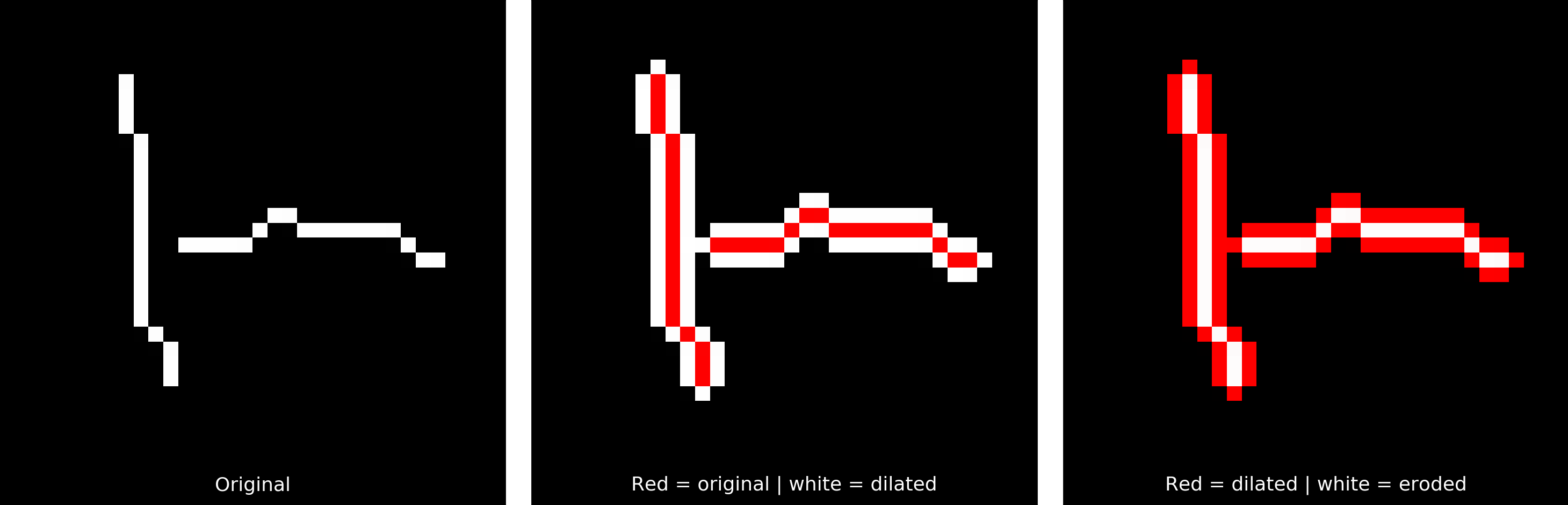
So we see that the edges do get linked by the dilation, but by only one pixel, which the following erosion then removes.
And now let’s break down the closing with disk of size two into its component. This is equivalent to applying two consecutive passes of dilation with disk of size 1, and then two consecutive passes of erosion with disk of size 1, as in the demonstration in the next figure below (by the way, if we observed carefully the second panel above we could predict that the dilation with a disk of size two would result in a link 3-pixel wide instead of 1-pixel wide, which the subsequent erosion will not disconnect).

Below is a GIF animated version of this demo, cycling to the above steps; you can also run it yourself by downloading and running the Jupyter notebook on GitHub.
Additional resources
Closing Jupyter notebook with complete Python code on GitHub
sketch2model Jupyter notebook with complete Python code on GitHub
More reading on Closing, with examples
Related Posts
sketch2model (2015 Geoscience Hackathon, Calgary)
